Proximity Analysis

N closest things. Things within x distance of this. Things that are within another. Both 2 and 3d geometries, 2d geodetic (aka geography), and even raster.

Example N-Closest using Geography data type

Closest 5 restaurants to here and kind of cuisine

SELECT 
    name, 
    tags->>'cuisine' As cuisine,  
    ST_Point(-74.036,40.724)::geography <-> geog As dist_meters
FROM nj_pois As pois
WHERE tags @> '{"amenity":"restaurant"}'::jsonb
ORDER BY dist_meters
LIMIT 5;
                        

name                         | cuisine               | dist_meters
-----------------------------+-----------------------+-----------------
Chilis                       | mexican               | 183.749762473017
Battello                     | italian               |  337.82552535307
Park and Sixth               | american              | 631.058208835878
Taphouse                     | NULL                  | 740.060280459834
The Kitchen at Grove Station | seasonal new american | 764.554569258853
                        

Geography within 1000 meters of location

Works for geometry as well, but measurements and coordinates are in units of the geometry, not always meters.

SELECT name, tags->>'amenity' As type, tags->>'cuisine' AS cuisine, ST_Distance(pois.geog,ref.geog) As dist_m
FROM nj_pois AS pois, 
	(SELECT ST_Point(-74.036,40.724)::geography) As ref(geog)
WHERE tags ? 'cuisine' AND ST_DWithin(pois.geog,ref.geog,1000)
ORDER BY dist_m;
                        

name                         | type       | cuisine               | dist_m
-----------------------------+------------+-----------------------+-------------
Chilis                       | restaurant | mexican               | 183.54545201
Battello                     | restaurant | italian               | 338.39714681
Starbucks                    | cafe       | coffee_shop           | 350.25322227
Park and Sixth               | restaurant | american              | 632.12204878
Torico Ice Cream             | fast_food  | ice_cream             | 741.32599554
The Kitchen at Grove Station | restaurant | seasonal new american | 764.72996783
Rustique                     | restaurant | italian               | 822.04122537
Helen's Pizza                | restaurant | pizza_Italian         | 866.65681852
                        

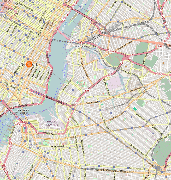
How many subway stops in each borough?

SELECT b.boro_name, COUNT(s.stop_id) As num_stops
FROM nyc_boros AS b INNER JOIN nyc_subways_stops AS s ON ST_Covers(b.geom,s.geom)
GROUP BY b.boro_name
ORDER BY b.boro_name;
                        

boro_name     | num_stops
--------------+----------
Bronx         |        70
Brooklyn      |       169
Manhattan     |       151
Queens        |        82
Staten Island |        21
                        

Proximity with 3D data

If you have things like oil pipe lines and using linestrings with a Z component, it's just like ST_Distance, except you want to use ST_3DDistance, ST_3DDWithin, and ST_3DIntersects. These are part of the core postgis extension.

For more advanced 3d, like if you need ST_3DIntersection, and ST_3DIntersects that does true surface and solid analysis (PolyhedralSurfaces), you'll want to install extension postgis_sfcgal.

Intersect raster and geometry: Raster value at a geometric point

SELECT pois.name, ST_Value(e.rast,1,pois.geom) AS elev 
FROM  pois INNER JOIN nj_ned As e ON ST_Intersects(pois.geom,e.rast)
WHERE pois.tags ? 'cuisine'
ORDER BY ST_SetSRID(ST_Point(-74.036,40.724),4269) <-> pois.geom
LIMIT 5;
                        

name                         | elev
-----------------------------+-----------------
Chilis                       | 2.64900875091553
Starbucks                    | 2.61004424095154
Battello                     | 2.18213820457458
Park and Sixth               | 3.79218482971191
The Kitchen at Grove Station | 2.06850671768188
                        

Reproject on-the-fly

Database column type transformation and conversion for geometry and geography

Convert from current projection to NYC State Plane feet (look in spatial_ref_sys for options).

ALTER TABLE nyc_boros 
ALTER COLUMN geom TYPE geometry(Multipolygon, 2263) 
USING ST_Transform(geom,2263);
                        

Convert geometry to geography

ALTER TABLE nyc_boros 
ALTER COLUMN geom TYPE geography(Multipolygon,4326) 
USING ST_Transform(geom,4326)::geography;
                        

Convert back to geometry

ALTER TABLE nyc_boros 
ALTER COLUMN geom TYPE geometry(Multipolygon, 2263) 
USING ST_Transform(geom::geometry,2263);
                        

ST_Transform for raster

For more info, read the manual http://postgis.net/docs/RT_ST_Transform.html. The algorithm defaults to NearestNeighbor algorithm, fastest but not the most appealing

SELECT ST_Transform(rast,3424) AS rast
FROM nj_ned 
WHERE ST_Intersects(rast,ST_SetSRID(ST_Point(-74.036,40.724),4269));
                        

You can override the warping algorithm

SELECT ST_Transform(rast,3424,'Lanczos') AS rast
FROM nj_ned 
WHERE ST_Intersects(rast,ST_SetSRID(ST_Point(-74.036,40.724),4269));
                        

Creating a whole new transformed table, align your rasters. This ensures rasters have same grid and pixel size.

WITH a AS (SELECT ST_Transform(rast,3424, 'Lanczos') AS rast
FROM nj_ned LIMIT 1)
SELECT rid, ST_Transform(n.rast,a.rast,'Lanczos') AS rast
INTO nj_ned_3424
FROM nj_ned AS n, a;
                        

3D Visualization

X3D useful for rendering PolyhedralSurfaces and Triangular Irregulated Networks (TINS), PolyHedralSufaces for things like buildings. TINS for Terrain

Checkout https://github.com/robe2/node_postgis_express built using NodeJS and http://www.x3dom.org (X3D in html 5)

3D Proximity and rendering

Use 3D bounding box &&& operator and form a 3D box filter

SELECT string_agg('<Shape><Appearance><ImageTexture url=''"images/' 
    || use || '.jpg"'' /></Appearance>' || ST_AsX3D(geom) || '</Shape>', '')
FROM data.boston_3dbuildings
WHERE 
    geom 
    &&& 
    ST_Expand(ST_Force3D(
        ST_Transform(ST_SetSRID(ST_Point(-71.0596787, 42.3581945),4326),2249))
        ,1000);
                        

X3Dom with texture

Address Standardization / Geocoding / Reverse Geocoding

PostGIS 2.2 comes with extension address_standardizer. Also included since PostGIS 2.0 is postgis_tiger_geocoder (only useful for US).

In works improved address standardizer and worldly useful geocoder - refer to: https://github.com/woodbri/address-standardizer

Address Standardization

Need to install address_standardizer, address_standardizer_data_us extensions (both packaged with PostGIS 2.2+). Using json also to show fields

SELECT *
FROM json_each_text(
    to_json(
        standardize_address('us_lex', 'us_gaz','us_rules',
    '29 Fort Greene Pl', 'Brooklyn, NY 11217'))
    ) WHERE value > '';
                        

key       | value
----------+------------
city      | BROOKLYN
name      | FORT GREENE
state     | NEW YORK
suftype   | PLACE
postcode  | 11217
house_num | 29
                        

Same exercise using the packaged postgis_tiger_geocoder tables that standardize to abbreviated instead of full name

SELECT *
FROM json_each_text( to_json(
    standardize_address('tiger.pagc_lex','tiger.pagc_gaz','tiger.pagc_rules', 
    '29 Fort Greene Pl','Brooklyn, NY 11217'))) WHERE value > '';
                        

key       | value
----------+------------
city      | BROOKLYN
name      | FORT GREENE
state     | NY
suftype   | PL
postcode  | 11217
house_num | 29
                        

Geocoding using PostGIS tiger geocoder

Given a textual location, ascribe a longitude/latitude. Uses postgis_tiger_geocoder extension requires loading of US Census Tiger data.

SELECT pprint_addy(addy) As address, ST_X(geomout) AS lon, ST_Y(geomout) As lat, rating
FROM geocode('29 Fort Greene Pl, Brooklyn, NY 11217',1);
                        

address                               | lon              | lat              | rating
--------------------------------------+------------------+------------------+-------
29 Fort Greene Pl, New York, NY 11217 | -73.976819945824 | 40.6889624828967 |      8
                        

Reverse Geocoding

Given a longitude/latitude or GeoHash, give a textual description of where that is. Using postgis_tiger_geocoder reverse_geocode function

SELECT pprint_addy(addrs) AS padd, array_to_string(r.street,',') AS cross_streets
FROM reverse_geocode(ST_Point(-73.9768,40.689)) AS r, unnest(r.addy) As addrs;
                        

padd                                  | cross_streets
--------------------------------------+---------------------
29 Fort Greene Pl, New York, NY 11217 | Dekalb Ave,Fulton St
                        

Photoshop with PostGIS

Pictures are rasters. Rasters are pictures. You can manipulate them en masse using the power of PostGIS raster.

Reading pictures stored outside of the database: Requirement

new in 2.2 GUCS generally set on DATABASE or system level using ALTER DATABASE SET or ALTER SYSTEM. In PostGIS 2.1 and 2.0 needed to set these as Server environment variables.

SET postgis.enable_outdb_rasters TO true; 
SET postgis.gdal_enabled_drivers TO 'GTiff PNG JPEG';
                        

Register your pictures with the database: Out of Db

You could with raster2pgsql the -R means just register, keep outside of database:

raster2pgsql -R /data/Dogs/*.jpg -F pics | psql

OR

CREATE TABLE pics (file_path text);
COPY pics FROM PROGRAM 'ls /data/Dogs/*.jpg';
ALTER TABLE pics ADD COLUMN rast raster;
ALTER TABLE pics ADD COLUMN file_name text;

-- Update record to store reference to picture as raster, and file_name
UPDATE pics SET rast = ST_AddBand(NULL::raster, file_path, NULL::int[]), 
    file_name = split_part(file_path,'/',4);
                        

Get basic raster stats

This will give width and height in pixels and the number of bands. These have 3 bands corresponding to RGB channels of image.

SELECT file_name, ST_Width(rast) As width, ST_Height(rast) As height, 
    ST_NumBands(rast) AS nbands
FROM pics
WHERE file_name LIKE 'd%';
                        

file_name            | width | height | nbands
---------------------+-------+--------+-------
dalmatian.jpg        |   200 |    300 |      3
doberman-pincher.jpg |   600 |    450 |      3
                        

Resize them and dump them back out

This uses PostgreSQL large object support for exporting. Each picture will result in a picture 25% of original size

SET postgis.gdal_enabled_drivers TO 'PNG JPEG';

DROP TABLE IF EXISTS tmp_out ;

CREATE TABLE tmp_out AS 
SELECT lo_from_bytea(0, ST_AsPNG(ST_Resize(rast,0.25, 0.25))) AS loid, filename
FROM pics;

SELECT lo_export(loid, '/tmp/' || file_name || '-25.png')
FROM tmp_out;

SELECT lo_unlink(loid)
FROM tmp_out;
                        

25% resized image

dalmation.jpg

dalmation.jpg-25.png

Change the pixel band values

A raster is an array of numbers. ST_Reclass lets you change the actual numbers by reclassifying them into ranges. This for example will allow you to reduce a 256 color image to 16 colors or change black spots to white spots.

WITH c AS (SELECT '(241-255:15, '  || string_agg(i::text || 
    ':' || (255-i)::text,',') AS carg 
    FROM generate_series(1,255) AS i) 
SELECT 
    ST_Reclass(
        rast,
        ROW(1,c.carg,'8BUI',255)::reclassarg, 
        ROW(2,c.carg,'8BUI',255)::reclassarg, 
        ROW(3,c.carg, '8BUI',255)::reclassarg
    ) AS rast
FROM pics, c
WHERE file_name = 'dalmatian.jpg';
                        

Dalmation Reversed

Before Reclass

After Reclass

Crop them

ST_Clip is the most commonly used function in PostGIS for raster. Here we buffer by 120 pixels from centroid of the picture and use that as our clipping region.

SELECT ST_Clip(rast, 
    ST_Buffer(ST_Centroid(rast::geometry), 120), 
    '{0,0,0}'::integer[])
FROM pics
WHERE file_name = 'dalmatian.jpg';

Dalmation Cropped

Before Crop

After Crop

Raster: Analyze Environmental Data

• Elevation
• Soil
• Weather

Min, max, mean elevation along a road

There are several stats functions available for raster. You'll almost always want to use these in conjunction with ST_Clip and ST_Count.

WITH estats AS 
 (SELECT sld_name, ST_Count(clip) AS num_pixels, ST_SummaryStats(clip) AS ss
FROM 
    nj_ned AS e INNER JOIN 
    (SELECT sld_name, geom 
        FROM nj_roads 
        WHERE sld_name IN( 'I-78', 'I-78 EXPRESS') ) AS r 
            ON ST_Intersects(geom, rast)
    , ST_Clip(e.rast, r.geom) AS clip
)
SELECT sld_name, MIN((ss).min) As min, MAX((ss).max) As max, 
    SUM((ss).mean*num_pixels)/SUM(num_pixels) AS mean
FROM estats
GROUP BY estats.sld_name;

   sld_name   |        min         |       max        |       mean
--------------+--------------------+------------------+------------------
 I-78         |  -6.32061910629272 | 298.695068359375 | 82.9211996035217
 I-78 EXPRESS | -0.877017498016357 | 97.2313003540039 | 30.5347544396378
(2 rows)
Time: 422.456 ms

Manage discontinuous date time ranges with PostGIS

A linestring can be used to represent a continous time range (using just X axis). A multi-linestring can be used to represent a related list of discontinous time ranges. PostGIS has hundreds of functions to work with linestrings and multilinestrings.

Helper function for casting linestring to date ranges

CREATE FUNCTION to_daterange (x geometry)
RETURNS daterange AS
$$
DECLARE
    y daterange;
    x1 date;
    x2 date;
BEGIN
    x1 = CASE WHEN ST_X(ST_StartPoint(x)) = 2415021 THEN '-infinity' ELSE 'J' || ST_X(ST_StartPoint(x)) END;
    x2 = CASE WHEN ST_X(ST_ENDPoint(x)) = 2488070 THEN 'infinity' ELSE 'J' || ST_X(ST_EndPoint(x)) END;
    y = daterange(x1, x2, '[)');
    RETURN y;
END;
$$
  LANGUAGE plpgsql IMMUTABLE;
                        

Helper function for casting date range to linestring

CREATE FUNCTION to_linestring (x daterange)
RETURNS geometry AS
$$
DECLARE
    y geometry(linestring);
    x1 bigint;
    x2 bigint;
    
BEGIN

    x1 = to_char(CASE WHEN lower(x) = '-infinity' THEN '1900-1-1' ELSE lower(x) END, 'J')::bigint;
    x2 = to_char(CASE WHEN upper(x) = 'infinity' THEN '2100-1-1' ELSE upper(x) END, 'J')::bigint;
    y = ST_GeomFromText('LINESTRING(' || x1 || ' 0,' || x2 || ' 0)');
    RETURN y;

    END;
$$
LANGUAGE plpgsql IMMUTABLE;
                        

Collapsing overlapping date ranges

Result is single linestring which maps to date range

SELECT id, 
    to_daterange(
        (ST_Dump(
            ST_Simplify(ST_LineMerge(ST_Union(to_linestring(period))),0))
        ).geom)
FROM (
    VALUES
        (1,daterange('1970-11-5'::date,'1980-1-1','[)')),
        (1,daterange('1990-11-5'::date,'infinity','[)')),
        (1,daterange('1975-11-5'::date,'1995-1-1','[)'))
) x (id, period)
GROUP BY id;
                        

 
id | to_daterange
---+----------------------
 1 | [1970-11-05,infinity)
                        

Collapsing discontinuous / overlapping ranges

Result is a multi-linestring which we dump out to get individual date ranges

SELECT id, 
    to_daterange(
        (ST_Dump(
            ST_Simplify(ST_LineMerge(ST_Union(to_linestring(period))),0))
        ).geom)
FROM (
    VALUES
        (1,daterange('1970-11-5'::date,'1975-1-1','[)')),
        (1,daterange('1980-1-5'::date,'infinity','[)')),
        (1,daterange('1975-11-5'::date,'1995-1-1','[)'))
) x (id,  period)
GROUP BY id;
                        

id | to_daterange
---+------------------------
 1 | [1970-11-05,1975-01-01)
 1 | [1975-11-05,infinity)
                        

Collapsing contiguous date ranges

Result is a linestring which we dump out to get individual date range

SELECT id, 
    to_daterange(
        (ST_Dump(
            ST_Simplify(ST_LineMerge(ST_Union(to_linestring(period))),0))
        ).geom)
FROM (
    VALUES
        (1,daterange('1970-11-5'::date,'1975-1-1','[)')),
        (1,daterange('1975-1-1'::date,'1980-12-31','[)')),
        (1,daterange('1980-12-31'::date,'1995-1-1','[)'))
) x (id,  period)
GROUP BY id;
                        

id | to_daterange
---+------------------------
 1 | [1970-11-05,1995-01-01)
                        

Create an Aggregate Function

CREATE OR REPLACE FUNCTION utility.collapse_periods_final(param_g geometry)
    RETURNS daterange[] AS
$$
     SELECT array_agg(a) FROM (SELECT to_daterange(
        (ST_Dump(ST_Simplify(ST_LineMerge(param_g),1))).geom)) AA a(a);
$$
LANGUAGE 'sql';

CREATE AGGREGATE utility.collapse_periods(daterange) (
    SFUNC=utility.linestring_add_daterange,
    STYPE=geometry,
    FINALFUNC=utility.collapse_periods_final, INITCOND='LINESTRING EMPTY'
);

CREATE OR REPLACE FUNCTION utility.linestring_add_daterange(c geometry,x daterange)
    RETURNS geometry AS
$$
     SELECT ST_Union(c,to_linestring(x));
$$
LANGUAGE 'sql';
                        

SELECT id, unnest(collapse_periods(period))
FROM (
    VALUES
        (1,daterange('1970-11-5'::date,'1975-1-1','[)')),
        (1,daterange('1980-1-5'::date,'infinity','[)')),
        (1,daterange('1975-11-5'::date,'1995-1-1','[)'))
) x (id, period)
GROUP BY id;                    
                        

id | to_daterange
---+------------------------
 1 | [1970-11-05,1975-01-01)
 1 | [1975-11-05,infinity)
                        

Super Collapse

WITH z (id,x,grade) AS (
    VALUES
        ('alex',to_linestring(daterange('2017-1-2','2017-1-3','[)')),'A'),
        ('alex',to_linestring(daterange('2017-1-1','2017-1-6','[)')),'B'),
        ('alex',to_linestring(daterange('2017-1-5','2017-1-8','[)')),'C'),
        ('alex',to_linestring(daterange('2017-1-1','2017-1-9','[)')),'X'),
        ('beth',to_linestring(daterange('2017-1-1','2017-1-3','[)')),'A'),
        ('beth',to_linestring(daterange('2017-1-5','2017-1-9','[)')),'B'),
        ('beth',to_linestring(daterange('2017-1-1','2017-1-9','[)')),'X')
) 
SELECT 
    a.id,
    to_daterange(a.u) AS period,
    MIN(b.grade) AS grade
FROM
    (SELECT id, (ST_Dump(ST_Union(x))).geom AS u FROM z GROUP BY id) a 
    INNER JOIN 
    z b
    ON a.id = b.id AND ST_Intersects(a.u,b.x) AND NOT ST_Touches(a.u,b.x)
GROUP BY a.id, a.u                
                        

 id   | period                  | grade
------+-------------------------+------
 alex | [2017-01-01,2017-01-02) | B
 alex | [2017-01-02,2017-01-03) | A
 alex | [2017-01-03,2017-01-05) | B
 alex | [2017-01-05,2017-01-06) | B
 alex | [2017-01-06,2017-01-08) | C
 alex | [2017-01-08,2017-01-09) | X
 beth | [2017-01-01,2017-01-03) | A
 beth | [2017-01-03,2017-01-05) | X
 beth | [2017-01-05,2017-01-09) | B
(9 rows)                
                        

WITH 
    z (id,x,grade) AS (
        VALUES
        ('alex',to_linestring(daterange('2017-1-2','2017-1-3','[)')),'A'),
        ('alex',to_linestring(daterange('2017-1-1','2017-1-6','[)')),'B'),
        ('alex',to_linestring(daterange('2017-1-5','2017-1-8','[)')),'C'),
        ('alex',to_linestring(daterange('2017-1-1','2017-1-9','[)')),'X'),
        ('beth',to_linestring(daterange('2017-1-1','2017-1-3','[)')),'A'),
        ('beth',to_linestring(daterange('2017-1-5','2017-1-9','[)')),'B'),
        ('beth',to_linestring(daterange('2017-1-1','2017-1-9','[)')),'X')
    ), 
    w AS (
        SELECT 
            a.id,
            a.u AS x,
            MIN(b.grade) AS grade
        FROM
            (SELECT id, (ST_Dump(ST_Union(x))).geom AS u FROM z GROUP BY id) a 
            INNER JOIN 
            z b
            ON a.id = b.id AND ST_Intersects(a.u,b.x) AND NOT ST_Touches(a.u,b.x)
        GROUP BY a.id, a.u
    )

SELECT
    id,
    to_daterange(
        (
            ST_Dump(
                ST_Simplify(
                    ST_LineMerge(
                        ST_Collect(x)
                    )
                    ,
                    0
                )
            )
        ).geom
    ) AS period,
    grade
FROM w
GROUP BY id, grade
ORDER BY id, period, grade
                        

id   | period                  | grade
-----+-------------------------+------
alex | [2017-01-01,2017-01-02) | B
alex | [2017-01-02,2017-01-03) | A
alex | [2017-01-03,2017-01-06) | B
alex | [2017-01-06,2017-01-08) | C
alex | [2017-01-08,2017-01-09) | X
beth | [2017-01-01,2017-01-03) | A
beth | [2017-01-03,2017-01-05) | X
beth | [2017-01-05,2017-01-09) | B
8 rows)
                        

Routing with pgRouting

Finding least costly route along constrained paths like roads, airline routes, driving distance analysis, fleet routing based on time constraints, and many more.

Buy our upcoming book (Feature complete Preview Edition available) pgRouting: A Practical Guide http://locatepress.com/pgrouting

to find out more

Traveling Sales Person problem

Routing nuclear power plant inspector

WITH 
    T AS (SELECT * 
        FROM  pgr_eucledianTSP($$SELECT id, ST_X(geom) AS x, ST_Y(geom) AS y 
            FROM nuclear_power_plants$$, 19, 19)
        )
SELECT T.seq, T.node AS id, N.name, N.geom, N.country
    FROM T INNER JOIN nuclear_power_plants N ON T.node = N.id
ORDER BY seq;

 seq | id  |                    name                     |    country
-----+-----+---------------------------------------------+----------------
   1 |  19 | Dukovany Nuclear Power Station              | Czech Republic
   2 |  20 | Temelin Nuclear Power Station               | Czech Republic
   3 |  45 | Isar Nuclear Power Plant                    | Germany
   4 |  44 | Gundremmingen Nuclear Power Plant           | Germany
   5 |  46 | Neckarwestheim Nuclear Power Plant          | Germany
   6 |  47 | Philippsburg Nuclear Power Plant            | Germany
   :
 150 |  55 | Higashidōri Nuclear Power Plant             | Japan
 151 |  64 | Tomari Nuclear Power Plant                  | Japan
 152 |  19 | Dukovany Nuclear Power Station              | Czech Republic
(152 rows)

Time: 48.706 ms

TSP in QGIS

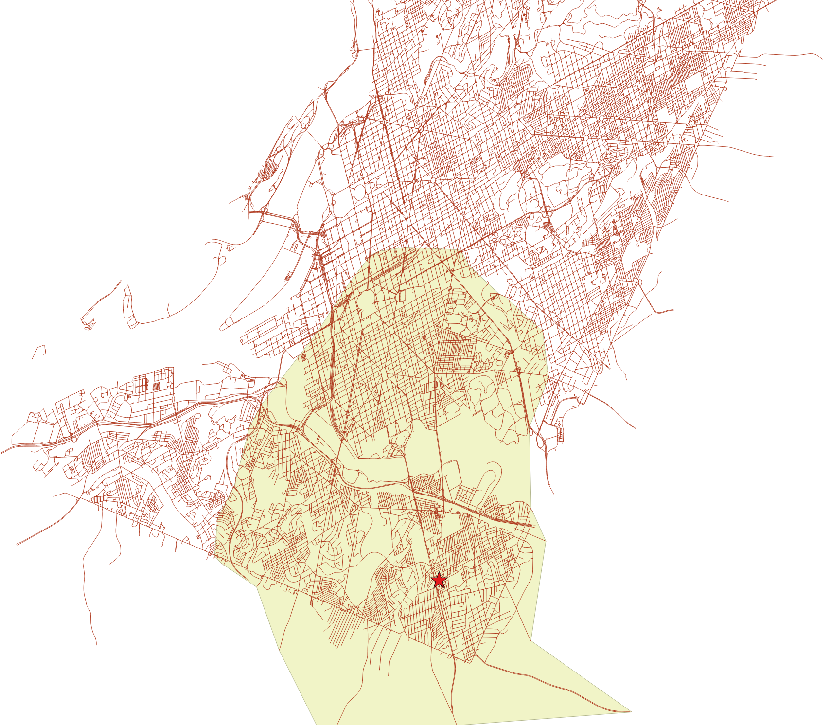
Catchment Areas: Drive Time Distance

What areas can a fire station service based on 5 minute drive time.

SELECT 1 As id, ST_SetSRID(pgr_pointsAsPolygon( 
    $$SELECT dd.seq AS id, ST_X(v.the_geom) AS x, ST_Y(v.the_geom) As y 
        FROM pgr_drivingDistance($sub$SELECT gid As id, source, target, 
            cost_s AS cost, reverse_cost_s AS reverse_cost 
            FROM ospr.ways$sub$,
        (SELECT n.id 
            FROM ospr.ways_vertices_pgr AS n
              ORDER BY ST_SetSRID(
                ST_Point(-76.933399,38.890703),4326) <-> n.the_geom LIMIT 1) 
        ,  5*60, true 
      ) AS dd INNER JOIN ospr.ways_vertices_pgr AS v ON dd.node = v.id$$
   ), 4326) As geom; 

Alphashape Area output in QGIS

Overlaid on roads network and with fire station location starred

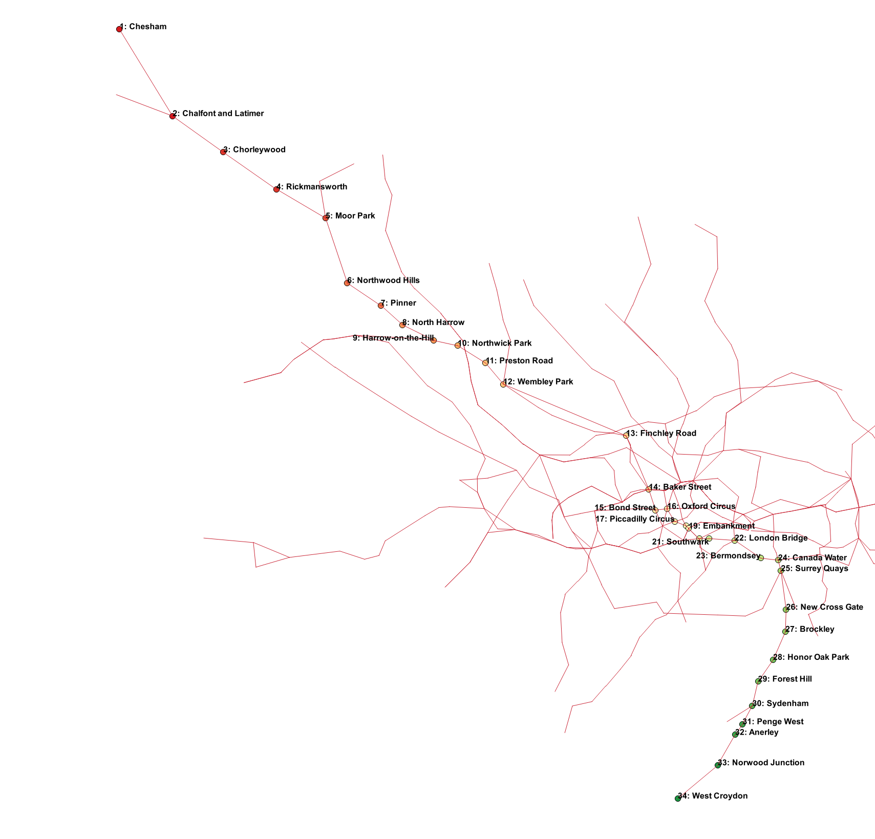
Dijkstra: Finding optimal route

Fastest path from Chesham to West Croydon

SELECT seq, S.station, L.name, round((cost * .000621371)::numeric,2) AS miles
FROM 
    pgr_dijkstra('
        SELECT gid AS id, source, target, length AS cost 
            FROM london_tube_lines',
        (SELECT station_id FROM london_stations WHERE station = 'Chesham'),
        (SELECT station_id FROM london_stations WHERE station = 'West Croydon'), 
        false
    ) R
    INNER JOIN london_stations S ON R.node = S.station_id
    LEFT JOIN london_tube_lines L ON R.edge = L.gid
ORDER BY R.seq;

 seq |       station        |     name     | miles
-----+----------------------+--------------+-------
   1 | Chesham              | Metropolitan |  3.38
   2 | Chalfont and Latimer | Metropolitan |  2.07
   3 | Chorleywood          | Metropolitan |  2.15
   :
  12 | Wembley Park         | Metropolitan |  4.42
  13 | Finchley Road        | Metropolitan |  1.93
  14 | Baker Street         | Jubilee      |  0.72
  :
  19 | Embankment           | Bakerloo     |  0.49
  20 | Waterloo             | Jubilee      |  0.33
  21 | Southwark            | Jubilee      |  0.86
  22 | London Bridge        | Jubilee      |  1.04
  23 | Bermondsey           | Jubilee      |  0.58
  24 | Canada Water         | Overground   |  0.37
 :
  31 | Penge West           | Overground   |  0.43
  32 | Anerley              | Overground   |  1.16
  33 | Norwood Junction     | Overground   |  1.72
  34 | West Croydon         | NULL         |  0.00
(34 rows)

Time: 36.509 ms

Dijkstra: Finding optimal route

London Tubes optimal path